Tuesday, April 29, 2008

Correctly reset LaTeX's theorem counters

Now that's a technical title to start with! Let's keep this short: I've gotten the following question a few times already. When numbering theorems (either standard LaTeX or by package amsthm) within sections (or deeper levels), the counter is not correctly reset when starting a new chapter (or in fact any level above your numbering level).

Example:

\newtheorem{lemma}{Lemma}[section]

\chapter{First chap}
\section{First sec}
\begin{lemma}that's the one\end{lemma}

\chapter{Second chap}
\begin{lemma}This number is wrong.\end{lemma}
\section{Next sec}
\begin{lemma}Now it's OK again.\end{lemma}

Will produce:
Chapter 1 First chap
1.1 First sec
Lemma 1.1.1 That's the one
Chapter 2 Second chap
Lemma 2.0.2 This number is wrong.

2.1 Next sec
Lemma 2.1.1 Now it's OK again.

Notice how the theorem counter did not get reset when entering the second chapter. It is only reset when entering a new section. Of course, I know that the zero is ugly, but apparantly some people really do want to include theorems in a chapter even before the first section has started.

Fix:
In your document preamble (after the \newtheorem), put the following:

\makeatletter
\@addtoreset{lemma}{chapter}
\makeatother

Note that this is only necessary for document classes report and book. When you are numbering within, e.g., subsection, also add a \@addtoreset{lemma}{section}. You'll get the idea.

Thursday, May 24, 2007

Two minor editor enhancements

Only for BibTeX and NEdit users: you probably know that the bibliography style often lowercases your texts for titles. This is not what you want in the following case:
An hllc riemann solver for magneto-hydrodynamics
You need to put braces around parts that should not be changed, i.e., in BibTeX form:
An {HLLC} {R}iemann solver for magneto-hydrodynamics
Put the following piece of code in your ~/.nedit/nedit.rc configuration file for NEdit.
nedit.macroCommands: \
...many built-in macros...
      }\n\
      BibTeX capitalise:Shift+Ctrl+U:c:R: {\n\
              replace_in_selection("([A-Z]+)", "\\\\{\\\\1\\\\}", "regex")\n\
      }\n
nedit.bgMenuCommands: \
After typing a title, just select it and press [Ctrl]+[Shift]+[U]. It will enclose all uppercase parts inside braces. Not much special about it, but handy it is. Oh, and whilst you have your configuration file open, also add this:
        Comments>% Comment@LaTeX:Shift+Ctrl+C:c:R: {\n\
                replace_in_selection("^.*$", "%&", "regex")\n\
        }\n\
        Comments>% Uncomment@LaTeX:Shift+Ctrl+Alt+C:u:R: {\n\
                replace_in_selection("(^[ \\\\t]*%)(.*)$", "\\\\2", "regex")\n\
        }\n\
When editing a LaTeX file, select some complete lines, press [Shift]+[Ctrl]+[C] and you'll have the entire block commented by % characters. Include the [Alt]-key to uncomment.

Thursday, April 26, 2007

Colorize your (svn) diffs

People who know me, know that I love color on my computer screen[1]. It helps me reading code or output faster. I was not on a side track today, no, but when cleaning up my ~/bin, I just thought that my tiny colordiff script may be useful to others too. It (modestly) colorizes output from svn diff, or plain diff output.

Here is an example of svn diff on a directory with some modified files:

[dam@doffer:~/avandam_svn/phd/sw/fortran/src]$ svn diff . | colordiff
Index: mmadapt.f
===================================================================
--- mmadapt.f   (revision 1114)
+++ mmadapt.f   (working copy)
@@ -429,8 +429,8 @@
subroutine eval_monitor
    integer :: i1, i2, iq, id
    real(knd_double) :: alphap(nq, ndim)
-       call eval_monitor_nondir
-       return
+       !call eval_monitor_nondir
+       !return

    call cellaverages(x, x, xc) ! I use this result in move_mesh too!

Index: mmsolve.f
[..]

You can also use this on normal diff output:

[dam@doffer:~/avandam_svn/phd/sw/fortran/src]$ diff mmadapt.f mmadapt_bla.f | colordiff plain
466c466
<               end do ! i2
---
>               end do ! i2 foo
485d484
<               dq(i1,i2,1:nq,1) = (q(i1+1,i2,1:nq) - q(i1-1,i2,1:nq)) / (xc(i1+1,i2,1) - xc(i1-1,i2,1))
503a503
>       ! bla

The colordiff script only uses sed and looks like this:

#!/bin/bash
# Mainly used to pipe output by 'svn diff' into
if [[ "$1" == "plain" ]] ; then # to use in plain diff usage
        sed -e 's/^\(>.*\)/ESC[1;34m\1ESC[0m/;s/^\(<.*\)/ESC[1;31m\1ESC[0m/;s/^\(diff .*\)/ESC[1;37;40m\1ESC[0m/'
else # for svn diff output
        sed -e 's/^\(\+.*\)/ESC[1;34m\1ESC[0m/;s/^\(\-.*\)/ESC[1;31m\1ESC[0m/;s/^\(Index: .*\)/ESC[1;37;40m\1ESC[0m/'
fi

sed just inserts the appropriate escape characters producing color output[2] at the right places. To make sure the escape characters are correct do not copy-paste, but download colordiff here.

[1] color output for Stratego.
[2] Escape characters producing color output.

Labels: , , ,

Wednesday, April 25, 2007

The Ultimate Coolness of Signal Catching

Patience is a virtue, but I seem to be lacking it. I often perform long computer simulations and continue working on my code when the program runs in a different window. The end result of the simulation is some data files containing the final solution.
What a waste of resources, however, when the simulation ends and it turns out to have become unstable in an early stage already, producing senseless data all the time. Or, imagine you really have to leave the office and want to take your laptop home, but the simulation is still only halfway. Pressing Ctrl-C is easy, but you'll have to start the simulation from the start again at home. I would like to save solution data at any intermediate time.
I decided to have a look at the use of UNIX signals to solve these little annoyances.

The idea is neither original, nor very difficult; it's just extremely handy! Most of my simulations consist of a large loop in the main routine that starts at simulation time Tstart and ends at time Tend, taking small time steps. Here's sample terminal output to get an idea:

[..]
#        1967  time =   0.1986020
finished MM after            2  steps (mmres=  9.5645049E-006 ).
#        1968  time =   0.1986853
finished MM after            2  steps (mmres=  9.8183985E-006 ).
[..]

When I press Ctrl-Z ('suspend'), this is what happens:

finished MM after            2  steps (mmres=  9.7805565E-006 ).
#        2594  time =   0.2427970  (Ctrl-Z pressed)
Caught suspend. Saving current data...
Continuing execution...
finished MM after            2  steps (mmres=  9.9850709E-006 ).
#        2595  time =   0.2428664

And when I press Ctrl-C ('interrupt'), this is what happens:

finished MM after            5  steps (mmres=  1.0567982E-005 ).
#        2617  time =   0.2444400 (Ctrl-C pressed)
Caught interrupt. Saving current data...
Exiting.

Note that I deliberately use the SIGINT (Ctrl-C) and SIGTSTP (Ctrl-Z) signals, because those are sent when pressing the stated key combinations. The reserved user signals SIGUSR1 and SIGUSR2 would have to be sent for example by the kill command, which is inconvenient for my use.

Implementation in Fortran

On UNIX systems, signal handling is performed by the functions defined in the system-wide (C-)library signal.h. Fortunately libsigwatch provides some basic but sufficient helper functions that allows us to define which signals we want to catch, and what special action should be taken.

Here is my relevant Fortran (95) source code:

module mmsignal
use mmio

contains

subroutine initsighandles()
  integer  watchsignal
  integer :: status
  status = watchsignal(2) ! SIGINT (Ctrl-C)
  status = watchsignal(20) ! SIGTSTP (Ctrl-Z)
  ! Optionally check for status == -1 to detect failure
end subroutine

subroutine catchsignals()
  integer getlastsignal
  integer :: lastsig

  lastsig = getlastsignal()

  if (lastsig .eq. 2) then
    print *, 'Caught interrupt. Saving current data...'
    call save_state
    print *, 'Exiting.'
    stop
  end if
  if (lastsig .eq. 20) then
    print *, 'Caught suspend. Saving current data...'
    call save_state
    print *, 'Continuing execution...'
  end if
end subroutine

end module

The routine watchsignal(int) installs special signal handling for the requested signal: each time the signal is received, it is stored in a variable accessible by calling the routine getlastsignal(). The custom signal handler itself is not handled by the sigwatch library: I call my own routine catchsignals() within the main loop's body that checks whether the most recent signal was either SIGINT or SIGTSTOP, and if not just does nothing.

To include the sigwatch library in your program, just add it to your linking stage and you are done:

> gfortran -lsigwatch finvol.o mmadapt.o mmbounds.o mmconfig.o mmdata.o mmio.o mmphys.o mmsignal.o mmsolve.o mmusr.o -o mmsolve

(Relevant parts are highlighted.)

Implementation in C(++)

In C++, we can directly use the functions in the (C-) signal library. I used this in a classroom package implementing genetic algorithms. The following code is incomplete, but all relevant parts are included:

#include <iostream>
#include <csignal>

#include "galib.h"

bool stopGiven = false;

void handleUserStop(int sig_num)
{
  stopGiven = true;
  std::cout << "*** User interrupt caught." << std::endl;
  std::cout << "*** Please stand by while current generation is completed and saved." << std::endl;
}

int main(int argc, char **argv)
{
  signal(SIGTSTP, handleUserStop);

  // ...

  while (!stopGiven) {
    p->nextGeneration();
    // ...
  }

  // In case of a user stop signal or when requested, save last generation
  if (stopGiven || parameters.savelastgen) {
    std::cout << "Writing generation #" << i << " to file \"" << LASTGENFILE << "\"." << std::endl;
    p->writePopulation(fpopout);
  }
  fpopout.close();

  delete p;
  return 0;
}

Notice how the custom signal handler now is enabled by the signal library, installed in one step by the call signal(SIGTSTP, handleUserStop);

Now that I have saved intermediate solution data, I can extend the main program to offer a resume functionality, using the data file for initialization. That task is not only easy, but it also does not have anything to do with signals, so I will not cover that here.

I still benefit from the above functionality almost every week, I hope it serves you well too.
Thursday, April 05, 2007

Cleaning up the Mesh

Allright, the following is intended only for a small public probably, but whoever occasionally puts pictures of adaptive meshes in electronic presentations should read on. I work with (moving) adaptive meshes. There is one major problem when visualizing these things: resolution. In printed matter, my EPS or PDF pictures exported from MATLAB are of course tack sharp. Unfortunately in small pictures, the hundreds of lines tend to blacken the entire image. Setting the line width to approximately 0.2 solves this.
» mh = mesh(x, y, 0*x, 'LineWidth', 0.2, 'EdgeColor', 'k');
That whas the easy part. Now what if the output device does not have as much resolution as a laser printer?

Mesh Moiré

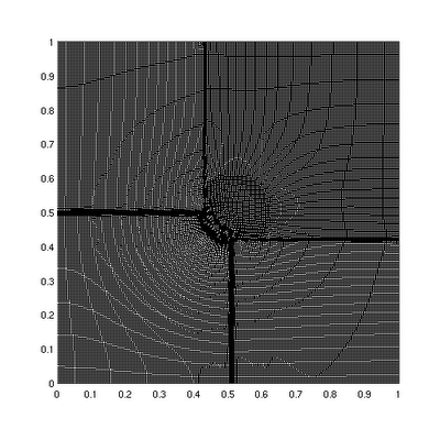
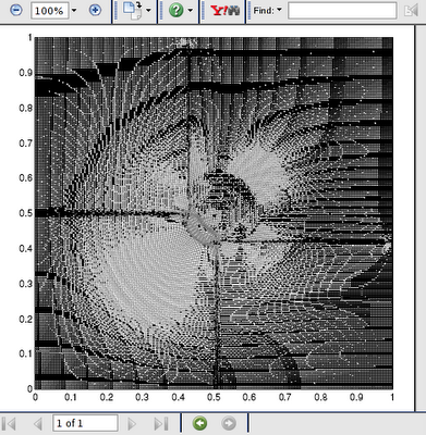
When using the same PDF pictures in an electronic presentation, e.g., by latex-beamer, the viewer is left to do a proper rendering of the vector graphics in the PDF picture at a low resolution (think of a 1024 px screen width). I have not seen a viewer do this without showing moiré effects. Below is a screen capture of acroread rendering a 200 by 200 adaptive mesh: It looks awful! This will not impress the audience! What makes this even more complicated is that each program performs differently (I've had the best results with acroread 4 so far...), and that at each location the beamer is probably different in resolution from prior locations. So, I wanted to get rid of the on site rendering of these vector graphics. I'll just create a bitmap version and include that. Here's the MATLAB PNG output: (Click on image for actual MATLAB output: MATLAB does not do antialiasing!) So, which program does do good rasterizing? I had heard Martin Bravenboer being really enthusiastic about the SVG rasterizer in the Batik SVG Toolkit. I got an SVG export for my MATLAB figure by the plot2svg add-on. In MATLAB, this was just:
» plot2svg('hd22conf11.svg')
Next, from a terminal, I let Batik render at the desired resolution:
> java -Xmx512m -jar $PKGROOT/batik/current/batik-rasterizer.jar -w 500 -h 500 -bg
 255.255.255.255 hd22conf11.svg
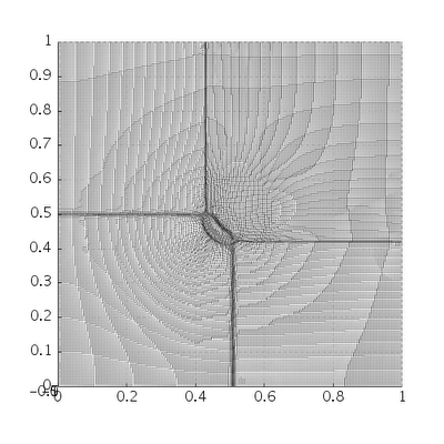
(Notice how I had to increase Java's maximum heap size; the SVG itself is 8MB, and the rasterizing apparently takes a lot of memory.) The resulting MATLAB -> SVG -> PNG output: Still far from optimal... I'm willing to lose some sharpness, if that rids me of the moiré. So, I rasterize a huge image, say 4000 by 4000 px, and scale that down to the desired size, e.g., by ImageMagick's convert:
> java -Xmx512m -jar $PKGROOT/batik/current/batik-rasterizer.jar -w 4000 -h 4000 -bg
 255.255.255.255 hd22conf11.svg
> convert -resize 500x500 hd22conf11.png hd22conf11_batik4000convert500.png
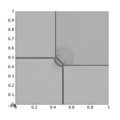
The resulting MATLAB -> SVG -> PNG large -> PNG resized output: Now, that's what makes me happy. Of course, some sharpness is lost, but what do you expect, for a 200 by 200 mesh on just slightly more than 400 by 400 px? A final note: when including the above PNG into your latex-beamer presentation will again lead to a resizing of this PNG, with minor moiré as a result. I found an image of 560 px wide, included at half size the most acceptable, and far better than anything I've seen so far.